Value of information

For a tutorial please see Value of Information tutorial.

Introduction

Value of information (VOI) is a powerful tool that allows us to perform diagnostics and troubleshooting.

Use cases

• Diagnosing a car or aircraft or autonomous vehicle
• Deciding whether a medicine is useful | see also Causal Optimisation
• Diagnosing a disease - also see Causal Inference
• A couuselling app
• etc..

Bayesian networks are built to support reasoning, diagnostics, causal inference and decision making, all under uncertainty. When we query a target (hypothesis) variable of interest, given any evidence (i.e. what we currently know about other variables), we are asking the model to calculate the so called posterior probability distribution for that target variable given any evidence. The returned distribution typically has some uncertainty associated with it. For example, if a variable X has states False and True, and X is currently False with probability 0.6 and True with probability 0.4, this is much less certain than if X is False with probability 0.1 and True with probability 0.9. The uncertainty (measured using Entropy), tells us how unsure we currently are about the state of a variable.

"Uncertainty is an uncomfortable position. But certainty is an absurd one" is a quote often attributed to French philosopher Voltaire, but attribution is disputed. But, most people want to make decisions without lots of uncertainty, and if we can reduce it, that is a good thing. This tool helps us.

Value of information

When encountering a problem, such as diagnosing a disease, it may be helpful to consult additional sources of information that could enhance the solution. (i.e. reduce the uncertainty in our target variable).

Value of information is a analysis tool, used to assess how beneficial new information could be before actually consulting the information source (e.g. performing an X-ray).

For example, this is ideal for guided diagnostics.

info

Bayes Server supports target or test variables that are discrete or continuous or a mixture of both.

info

For Decision Graphs, this can also take costs into account.

info

Value of information in Bayes Server uses a greedy target driven approach. What this means is that we only consider individual variables when seeking an improvedment to the target variable. We do not consider pairs of variables or more at each step.

Approach

Bayes Server uses an information theoretic approach to Value of information (entropy, mutual information and information gain).

Entropy and Mutual information

The primary reason for gathering additional information (evidence) is to reduce the uncertainty about the target (hypothesis) variable being evaluated. Choosing the next variable to observe (such as the next question to ask) can rely on the concept of Entropy. Entropy quantifies the extent to which the probability distribution of a variable is spread (over states for a discrete variable), serving as an indicator of randomness. The greater the randomness of a variable, the higher its entropy will be.

Entropy, often denoted $H(X)$, tells us how uncertain we are about the state of a variable. Value of Information seeks the next variable to observe, that will reduce this value the most.

Entropy:

$$H(\text{X}) = -\sum_{x}P(\text{X} = x) * ln( P(\text{X} = x))$$

info

For a discrete variable with $n$ states, entropy is highest, $ln(n)$, when the probability distribution is uniform. It is lowest, $0$, when the probability is 100% in a single state.

We can also measure how much entropy changes as new observations are made. If Y is another variable that we observe, then the updated entropy of X given Y can be calculated as follows:

$$\begin{align} H(X | Y ) = - \sum_{Y}P(Y) * \sum_{X}P(X | Y) * ln( P(X | Y)) \\ = H(X) - I(X,Y) \end{align}$$

where I(X,Y) is the Mutual information, a.k.a. cross entropy, of X and Y.

$H(X | Y)$ is known as the conditional entropy and is a measure of uncertainty of X given Y. Mutual information $I(X,Y)$ however, is the information shared between X and Y. Mutual information can be though of as the value of observing Y when the target of interest is X.

info

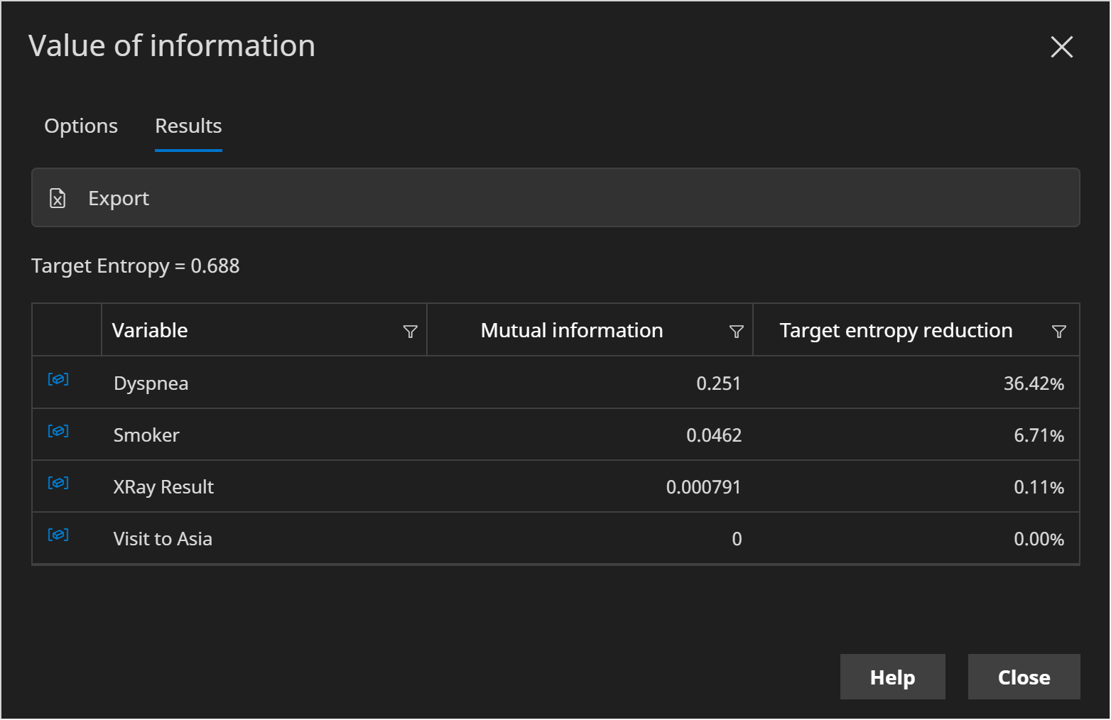
When we look at potential variables to observe, the higher the mutual information the better and therefore the User Interface automatically sorts by descending mutual information.

note

It is important to note, that the mutual information is the expected reduction in entropy, i.e. weighted by how likely each state in $Y$ is (for discrete variables). Therefore you may find the actual reduction achieved to much lower or higher, but since we do not know yet what the observed state of $Y$ will be, mutual information is a very useful measure.

Calculating Value of Information

Select the Target variable (sometimes referred to as the hypothesis variable). This is the variable whose uncertainty you want to reduce, for example the target of a troubleshooting system.

The Use current evidence check-box, when true, ensures that the calculations take into account any evidence currently set.

Click the Run button to perform the calculations. The Target entropy text displays the current level of uncertainty. And the table shows how other variables are likely to reduce that uncertainty in decreasing order.

info

One of the most useful columns is Target entropy reduction, which tells us the percentage by which the uncertainty metric is reduced.

Time series

There are a number of options which affect how the calculations are performed wth time series. These are explained below.

Consider a target variable H and a test variable T.

Target time

The Target time is the time (t) associated with the Target variable during the calculations.

info

The mutual information I(H[time = t];T) is calculated for H at time t. (Note that T could also have a time, if it is a temporal variable).

Test time

The Test time is the time (t) associated with the Test variable during the calculations.

info

The mutual information I(H;T[time=t]) is calculated for T at time t. (Note that H could also have a time, if it is a temporal variable).

Terminal time

If a time series model has any terminal nodes, a terminal time (absolute, zero based) is required. The terminal time determines the point at which Terminal nodes link to temporal nodes.