Junction Trees

Since version 11.0

The default Relevance Tree inference algorithm used by Bayes Server, is an exact inference algorithm. Internally it builds one or more data structures called Junction trees. These data structures provide an efficient way to calculate the requested queries given the current evidence. They are typically much more efficient than building the entire joint distribution, which is often intractable and if not, very slow.

However, junction trees typically consume more memory than the original node distributions. How much more, depends on the structure of the network, the current evidence and queries are being requested.

It can be important to understand these internal distributions, so you can analyze the performance of your network, or for teaching purposes. By understanding the internals, you can better understand why a query may be slow and how you may be able to refactor the network to improve performance.

info

It is important to note that in Bayes Server a junction tree is created dynamically and will therefore change depending on the following:

• Any evidence set
• Which nodes are being queried

Junction Tree construction

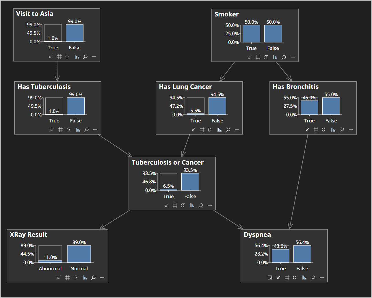
To understand junction trees, we will consider the Asia network, included as a sample with Bayes Server, shown below.

To simplify the equations, we use the following aliases to refer to variables:

Variable	Alias
Visit to Asia	A
Has Tuberculosis	T
Smoker	S
Has Lung Cancer	L
Has Bronchitis	B
Tuberculosis or Cancer	O
XRay Result	X
Dyspnea	D

The table below shows the distributions which are specified on each node:

Variable	Node distribution
A	P(A)
T	P(T|A)
S	P(S)
L	P(L|S)
B	P(B|S)
O	P(O|T,L)
X	P(X|O)
D	P(D|O,B)

Marginalization

We compute queries of interest by summing over (marginalizing) variables that are not in our final query. So, for exmaple if we had a distribution P(A,B,C) and we were interested in P(A) we would sum over B and C. This is denoted mathematically as $P(A) = \sum_{B,C}P(A,B,C)$

Full joint distribution

We could multiply all the distributions in the Asia network together and then use marginalization to calculate our queries, however with discrete variables the joint distribution grows exponentially with the number of variables.

We therefore build a data structure called a junction tree, which allows us to compute the same queries more efficiently. We can do this more efficiently thanks to the Distributive Law

Distributive Law

The Distributive Law which is part of standard probability theory, shown below, simply says that if we want to marginalize out a variable from a set of distributions, we only need to combine the distributions that contain that variable.

$$if A\notin \textbf{X},A\in \textbf{Y}, then \sum_A \phi_ \textbf{\tiny{X}}\phi_\textbf{\tiny{Y}}= \phi_ \textbf{\tiny{X}} \sum_A \phi_ \textbf{\tiny{Y}}$$

Where, $\phi$ is a set of distributions.

This simply means that if we want to marginalize out the variable $A$ we can perform the calculations on the subset of distributions that contain $A$.

info

This is the secret behind why inference in Bayesian network is so much more efficient and tractable that considering the joint distribution.

Elimination Order

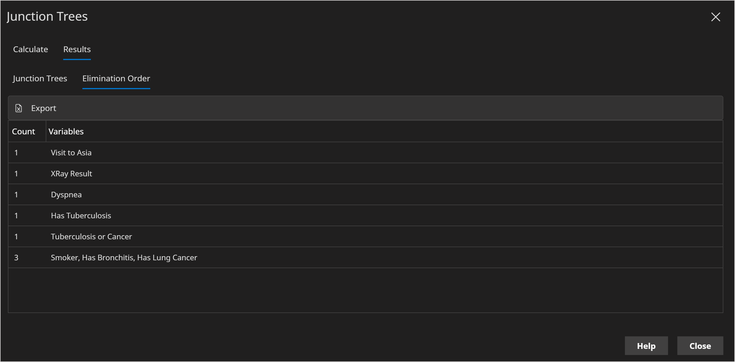
To build a junction tree, which can then be used to calculate the queries we require, we need to eliminate all relevant variables. Eliminating a variable means gathering up all distributions which contain that variable, multiplying them together and then marginalizing out that variable.

The order in which we eliminate variables will determine how efficient inference will be. There are a number of different algorithms to determine good elimination orders, which are out of scope for this article.

info

Note that sometimes multiple variables can be eliminated at the same time.

Once we have determined a good elimination order we have a data structure called a Junction Tree. Inference then proceeds in 2 phases, Collect and Distribute. Details of this procedure is out of scope for this article, but can be found in any text on Bayesian networks.

We can see in the image for the Asia network above that the first variable to be eliminated is Visit to Asia (A).

Consider the joint distribution over all variables (U).

$P(\textbf{U}) = P(A)P(T|A)P(S)P(L|S)P(B|S)P(O|T,L)P(X|O)P(D|O,B)$

In the above equation there are only 2 distributions that contain $A$, i.e. P(A) and P(T|A). To eliminate A we can multiply these together and marginalize out A.

$P(\textbf{U}) = (\sum_{A}P(A)P(T|A)) * P(S)P(L|S)P(B|S)P(O|T,L)P(X|O)P(D|O,B)$

Cliques and Sepsets

The distribution created when multiplying together P(A) and P(T|A) is called a Clique.

The distribution created after marginalizing out (summing over) A is called a Sepset and will no longer contain any variable(s) that have been eliminated (in this case only A).

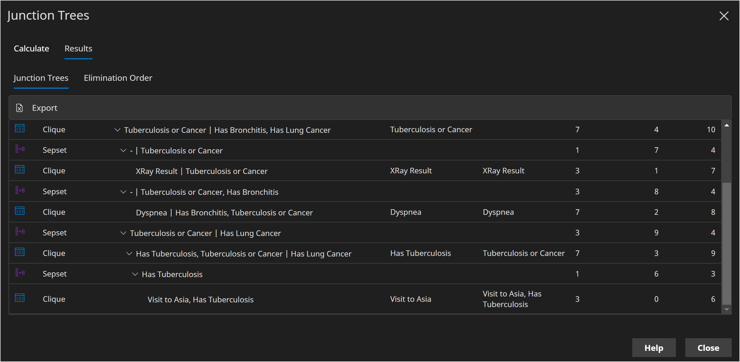
At the bottom of the image below, we can see the elimination we just performed.

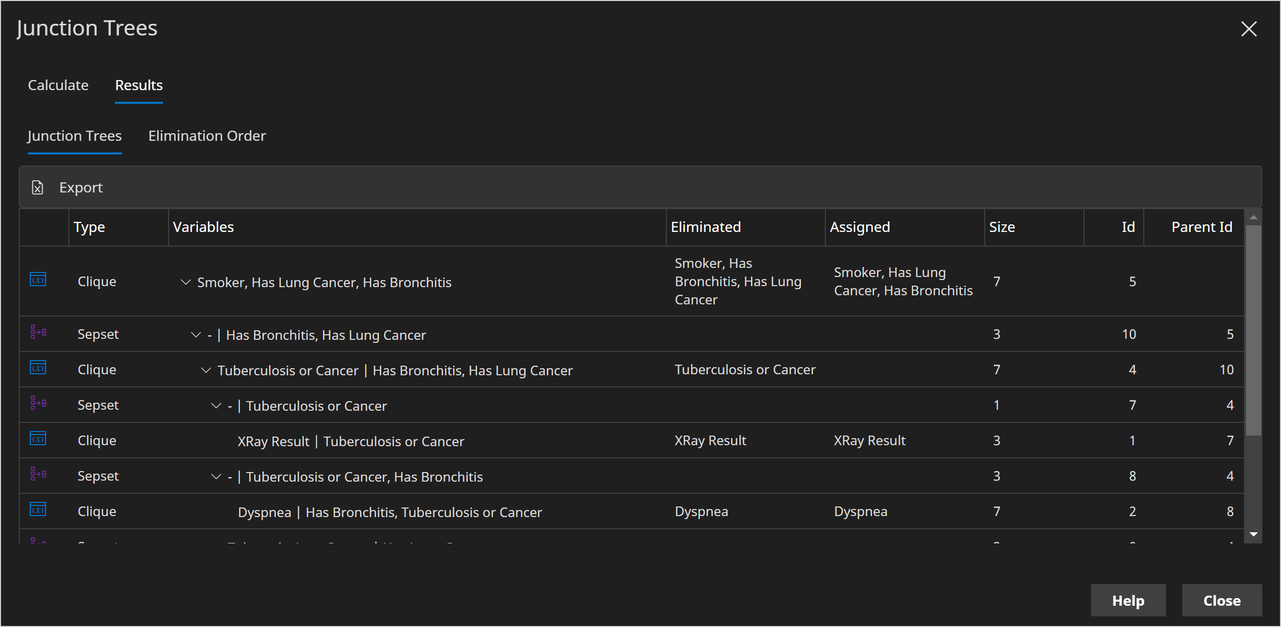
We can see that we eliminated A, the Clique contains A and T and the node distributions involved were P(A) and P(T|A). The size of the clique is 3 because P(A) * P(T|A) = P(T,A) has 4 values, but only 3 parameters as joint discrete distributions sum to 1 so one value can be calculated from the others.

Junction Tree Viewer Columns

• Variables | The list of variables in the Clique or Sepset
• Eliminated | Which variables have been eliminated at this step
• Assigned | Which node distributions are multiplied together to form the Clique
• Size | The size, in terms of parameters, of the Clique or Sepset

Multiple trees

There maybe be more than one junction tree for a number of reasons.

• Evidence or network structure makes groups of nodes independent of each other, therefore not needing to be in the same junction tree.
• A network is disconnected, i.e. has groups of nodes which have no links between them

Analysis

If we find that exact inference is intractable or slow, we can analyze the junction tree(s) to determine why.

info

Analyzing a junction tree is somewhat similar to analyzing a SQL query plan, which can help us understand why a SQL query is inefficient.

While Tree Width helps us understand the largest Clique, junction trees help us understand the individual Cliques and Sepsets that have a large number of parameters.

There are a number of ways we can reduce large Cliques.

• Divorcing
• Noisy nodes
• Reverse links (not always possible for causal networks )
• Reduce multiple paths in DBNs