Introduction to Causal AI
Correlation vs Causation
Many of us are familiar with the phrase 'correlation does not imply causation'. This correctly tells us that even if we know that there is an association (correlation) between a pair of variables (or sets of variables) this does not tell us anything about whether one variable (or set) causes another.
"If data shows that as the number of fires increase, so does the number of fire fighters. Therefore, to cut down on fires, you should reduce the number of fire fighters." - Pearl, Book of Why 2018
If correlation does not imply causation, then what is it?
This article provides a detailed introduction to the science of causal models, causal inference & causal optimization, which can be used to quantify this cause and effect relationship and make causal aware decisions based on observational data.
Causal analysis is used by policy/decision makers such as governments, heath-care policy makers, executive leaders and marketing analysts.
Often decision makers are making decisions based on BI dashboards and KPIs that do not consider causality, leading to either sub-optimal or worse incorrect decisions which can have severe financial implications or can even cost lives, as illustrated in this article.
Anyone making data driven decisions, should consider whether a causal analysis is required and the dangers of using non-causal decision making.
Observational Data
Observational data (also referred to as Real world evidence (RWE), especially in medicine) means data obtained outside the context of randomized controlled trials (RCTs). For example, data generated during routine clinical practice.
If you have conducted a randomized controlled trial (RCT) causal inference is not required.
RCTs are often not possible. for example:
- It may not be possible to subject a sub-population to a treatment -> effect of interest such as smoking -> cancer, as you can't ethically force people to smoke for a number of years.
- It may be too expensive to conduct an RCT
- You may wish to carry out many pre-RCT experiments to prioritize those most likely to succeed.
- The design of an RCT was found to contain bias, so we need to back-off to observational data.
Conditioning / stratification
When an RCT is not possible, statisticians will often examine subsets of data, by conditioning on a number of variables (known as stratification), and measure the cause-effect relationship within subsets, amd weight to get an overall statistic.
Unfortunately, without a causal analysis, it has been shown that while conditioning is often effective at closing off bias which would otherwise invalidate the cause-effect measurement, it can also open causal paths which can actually introduce bias.
D-Separation provides us with a means to determine whether there are any biasing paths given evidence, in complex networks. Colliders are a simple construct that illustrates how conditioning can introduce rather than reduce bias.
Fortunately a proper causal analysis alleviates the issues found when using conditioning/stratification, however it does require that we can agree on a causal structure (unless we are using the disjunctive cause criterion discussed later).
Interventions
When we enforce a new policy, we are overriding the normal behavior of people (or assets, etc...).
For example, a government policy to wear masks, overrides the normal reasons for wearing a mask, such as risk of exposure to pollutants or disease.
Overriding a variable is different to observing its behavior. When we override it is called an Intervention.
When we set standard (non-interventional) evidence all we are doing is narrowing the focus of our attention to a subset of the data (much like a SQL WHERE clause). However when we set interventional evidence we are actively changing the system, rather than just observing it.
When we set normal (non-interventional) evidence on a variable in a Bayesian network / causal model, information flows back up to its parents. For example, if we observe that someone is wearing a mask, without a government policy in place this behavior makes sense, because as we observe someone wearing a mask, it becomes more likely that individual is concerned about pollution and/or infection.
However when we set interventional evidence, the normal factors for wearing a mask are overridden, and information should therefore not flow to its parents in the normal way.
Note that when we conduct an RCTs, we are actually performing an intervention on the treatment group, so we do not need to perform causal inference, we can simply compare the treatment and non-treatment groups.
Terminology
Do operator
An intervention is often denoted with the Do operator. So if we are interested in the effect of a drug on recovery, since prescription of a drug is an intervention, we could denote this P(Recovered=True | Do(Drug)).
Treatment variable
A treatment variable in a causal analysis (or RCT) is the variable on which we intervene. For example, when performing a causal analysis on the effect of a Drug on Recovery, Drug is the intervention variable and hence the treatment.
Outcome variable
An outcome variable in a causal analysis (or RCT) is the variable which we are measuring the effect on. For example, when performing a causal analysis on the effect of a Drug on Recovery, Recovery is the outcome.
Confounder
A confounder is a common cause of both a treatment and an outcome.
A mathematical definition is any variable that makes P(Y | do(X)) differ from P(Y |X).
Confounders are important because they have the potential to bias a non-causal analysis. This is because in a non-causal analysis, information can flow back up from the treatment to the confounder and the subsequent change in the confounder can in turn effect the outcome. This is not what we want when we are trying to measure the effect of just the treatment in question.
Observed confounder - When a confounder is observable it is called an observed confounder.
Unobserved confounder - When a confounder is unobservable it is called an unobserved confounder.
When there are unobserved confounders present, we need to resort to methods that support them. We will cover them later in this article.
Backdoor
When information can pass from treatments back through confounders to the outcome this is known as a Backdoor. A common approach to causal analysis is to block all backdoor paths so we can measure the true cause-effect, but there are other clever approaches.
Covariate
Cause of treatment, cause of outcome, or both.
Mediators
Variables which fall on causal paths from treatment(s) to outcome(s).
Causal models
Before we walk-through a simple example of measuring the causal effect of an intervention, we need to ensure that we are using a Causal model. In the case of Bayes Server, the causal model will be a causal Bayesian network.
We will use the terms Causal model, Causal network, & Causal Bayesian network interchangeably.
Graphical approaches to Causality such as Bayesian networks and structural equation models are not the only approach for performing causal analysis, however we will be focusing on them in this article as they have become very popular, and increasingly so since the hugh success of the Book of Why (Judea Pearl et al. 2018).
A causal Bayesian network differs from a standard Bayesian network in that each directed link in a causal model implies a cause -> effect relationship, as opposed to just an association.
One notable exception to this is when we use the Disjunctive Cause Criterion which we will discuss later. This criterion does not require links to be causal.
Once we have established the directed causal links we can then proceed to a causal analysis.
The links in a causal network are often determined manually, however there are also techniques to perform what is known as causal discovery which are out of scope for this article.
Bayes Server supports both discrete and continuous variables in causal models.
Causal inference example
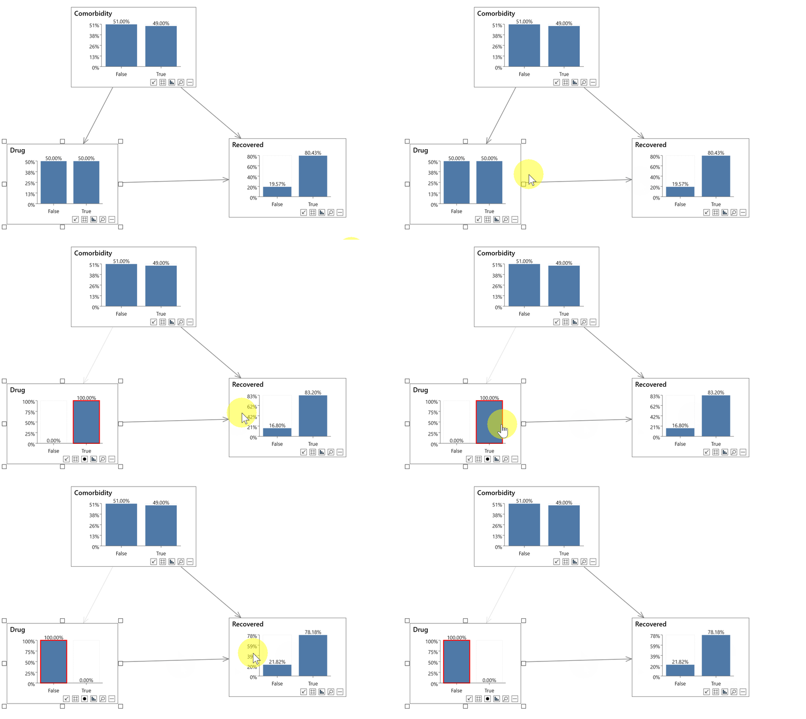
The simple causal model shown in the following animations contains 3 variables, Drug (the treatment), Recovered (the outcome) and Comorbidity (an observed confounder).
In this example we have a single treatment and a single outcome, but Bayes Server supports multiple treatments and multiple outcomes.
The example causal model is installed with Bayes Server, and is called Causal Inference Simple.
Non-causal analysis

In the first animation above we perform a non-causal analysis in an incorrect attempt to measure the effect of a Drug on Recovery rates.
- P(Recovered=True) = 80.43%
- P(Recovered=True|Drug=True) = 77.97%
- P(Recovered=True|Drug=False) = 82.89%
It looks like the drug is reducing the recovery rate by nearly 5%, which is incorrect.
Causal analysis

In the second animation above, instead of setting standard evidence on the Drug variable as in the non-causal analysis, we can instead perform an intervention.
A red border indicates an intervention, and incoming links are dimmed.
To set interventional evidence you can either:
- Right click a node, and click Do(state name) in the Evidence menu.
- Shift click on the node state
Performing the causal analysis we now see that:
- P(Recovered=True) = 80.43%
- P(Recovered=True|Do(Drug=True)) = 83.20%
- P(Recovered=True|Drug=False) = 78.18%
So the true causal effect of the drug is actually +5%, not -5%.
This is an example of Simpson's paradox, and a causal analysis allows us to resolve the paradox.
Explanation
Without performing the required intervention for a causal analysis, setting standard evidence on Drug causes information to flow back up to the confounder Comorbidity which in turn impacts Recovered. In this example the number of people with comorbidities varies greatly between those given the Drug and those who didn't which leads to the extreme difference between +5% and -5% seen in this example.
To properly measure the effect of Drug on Recovered we must block information flowing through the backdoor.
Even with less extreme differences between a causal and non-causal analysis it can still lead to the success or failure of a policy or even lives lost.
Note that Bayes Server supports interventions on discrete variables, continuous variables and even time series variables.
Causal optimization
Bayes Server supports Evidence optimization which is a powerful approach to automated decision making.
An alternative approach to Evidence Optimization for automated decision making is to use Decision graphs.
If among the input variables to our optimization there are policy decisions to make, such as which combination of drugs to chose based on cost & efficacy, we need to perform a causal aware optimization. i.e. policy variables need to have interventional evidence not standard evidence set on them during the optimization process.
Another way to describe Causal optimization is Causal Course of Action.
Causal optimization example
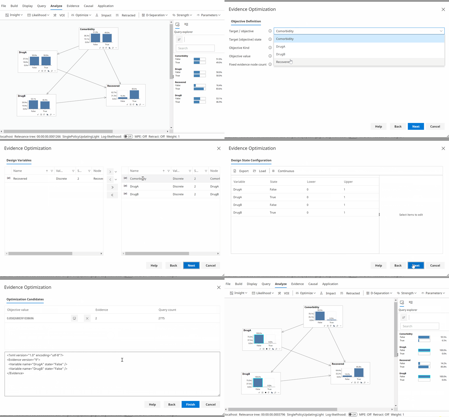
The simple causal model shown in the following animations contains 4 variables, DrugA (a treatment), DrugB (a treatment), Recovered (the outcome) and Comorbidity (an observed confounder).
The task in this example is to optimize the probability of recovery, P(Recovered=True).
The example causal model is installed with Bayes Server, and is called Causal Optimization Simple.
Non-causal analysis

In the first animation above we perform a non-causal analysis in an incorrect attempt to optimize the recovery rate, based on the the use or otherwise of 2 potential drugs.
Following a non-causal optimization, the analysis suggests we should not use either DrugA or DrugB (which is incorrect).
P(Recovered | Do(DrugA=False), Do(DrugB=False)) = 78.18% (Not 85.83% as reported by the optimization wizard as that does not use interventions!)
Causal analysis

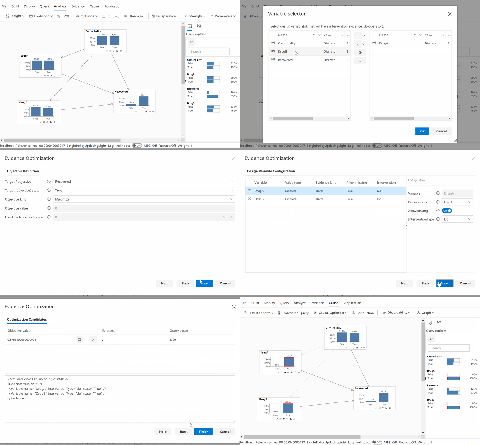
Instead of the optimization process considering standard evidence on DrugA and DrugB as in the non-causal analysis, we can instead allow interventions during the optimization as shown in the animation above.
Following a causal optimization, the analysis suggests we should use both DrugA and DrugB.
P(Recovered | Do(DrugA=True), Do(DrugB=True)) = 87.65%
Cost based optimization
Usually optimization includes costs. For example, unfortunately we cannot always afford to administer drugs even when they are known to be highly effective.
Bayes Server allows optimization of states, continuous variables and also functions.
We could easily extend this example to include costs, perhaps using a function node.
Counterfactuals
While interventions allow us to measure the causal effect of policy/actions from observational data, counterfactual analysis allows us to consider alternative realities (what would have happened?).
Another way to describe Counterfactual analysis is Causal What If? analysis.
Another useful distinction, is that interventions are analyzed on many rows of observational data, while counterfactual analysis is typically performed at the level of an individual row of data (such as an particular individual/event) or small group.
For example, on my drive home from work, would a different route have been quicker? It turns out that humans are very good at imagining and quantifying alternate realities, perhaps making use of similar past experiences, even if they have little or no past data relevant to the particular scenario.
Example & Calculation
Consider the following example from Pearl's Book of Why (2018, p273):
If salary is based on experience and education level (and luck? Connections, etc…), was it worth doing a PhD?
In a non-counterfactual analysis it may be tempting to simply change PhD to no PhD and look at similar data, and make a judgment on whether the PhD was worth doing. Unfortunately this would not take into account the work experience (often 6 years in the US) lost through doing the PhD. So you would be comparing the worker with a PhD to someone with 6 years less experience.
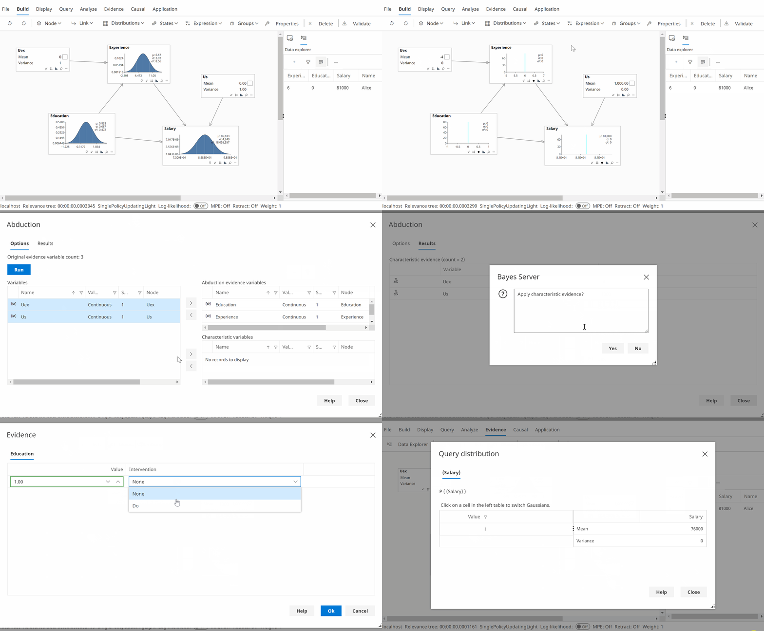
To perform a counterfactual analysis for Alice:
- Open the sample network Counterfactuals BOW, included with Bayes Server.
- Enter evidence for Alice [Experience=6, Education=0, Salary=81000].
- Use the Abduction dialog to calculate the characteristic variables Uex and Us, which will also remove the original evidence.
- Perform the intervention Do(Education=1).
- View Salary which now has the value 76000.
The animation below shows this calculation using Bayes Server (version 10 or later).
You can perform the same calculations with 9.4 or later, but some of the helper functions such as abduction are available from version 10 onwards.

Unobserved confounders
When there are no unobserved confounders present, the standard Bayes Server inference algorithms can perform inference with interventions present.
They do this by blocking the flow of information to parents of nodes with interventions set.
This is a so called backdoor adjustment on the parents of interventions.
Backdoor adjustments need not be on the parents, as long as they block the information flowing back to a confounder and through to the outcome(s).
Because a backdoor adjustment requires us to be able to condition (stratify) the data, we have a problem if unobserved confounders are present as we cannot condition on since we do not have data for them.
It turns out that when unobserved confounders are present there are additional methods we can employ to get round this limitation.
Often each approach has two stages. The first is an identification step called a criterion which uses algorithms to determine how a cause-effect relationship can be measured, the second is the measurement itself often referred to as an adjustment.
Often an expression containing the do-operator is converted to a do-free expression which can be calculated with standard inference.
Popular approaches are listed below, many of which are available from version 10 onwards in Bayes Server.
Backdoor criterion/adjustment - Identify variables that block back-door paths, and use the backdoor adjustment formula to calculate the effect. For a set Z of non-descendants of X that block certain paths from X to Y, then P(Y|do(x)) = _sum(z)( P(Y|z,x)P(z) )
Graph surgery - Equivalent to backdoor, adjusting for parents of interventions. (No unobserved confounders)
Front-door criterion/adjustment - Find a front-door path that is shielded from confounders – front door adjustment
Instrumental variables
Disjunctive Cause Criterion - a method which does not require links to be causal, so can make use of a standard Bayesian network and non-causal structural learning techniques. To use this method we need to be able to identify (and subsequently adjust for, using the Backdoor adjustment) all confounders (common causes) and that confounders are not unobserved.
Do-calculus - a lower level, but fully fledged calculus which can be tried when the criterion above cannot identify a way to proceed.
Note that it is not always possible to find a valid criterion and do-calculus may not help either.