Log Likelihood Tutorial

In this tutorial we will use the Waste sample network, which is included with Bayes Server, to demonstrate how to use the Log Likelihood query and Log-Likelihood batch query.

The log-likelihood helps us understand how unusual evidence is. We could use it to detect anomalies for example.

info

Bayes Server supports log-likelihood queries with both discrete and continuous variables (as well as time series).

The log-likelihood is the logarithm of the likelihood, where the likelihood in this context is the Probability of the current evidence $E$ denoted $P(E)$. The log-likelihood can therefore be written $log(P(E))$.

For purely discrete networks $P(E) \in{[0, 1]}$ and therefore $log(P(E)) \in{[-\inf, 0]}$ (although log(0) is often regarded as undefined).

For networks that include one or more continuous variables, $P(E) \in{[0, \inf]}$ and therefore $log(P(E)) \in{[-\inf, +inf]}$.

info

We tend to use the log-likelihood rather than the likelihood, because the likelihood can easily underflow (reach zero quickly), whereas the log-likelihood helps us measure with greater precision and is therefore better for handling and comparing extreme/anomalous data.

Part 1 - Single log-likelihood query

• Open the Waste sample network included with Bayes Server, either from the Start Page or from the File menu, click Open.

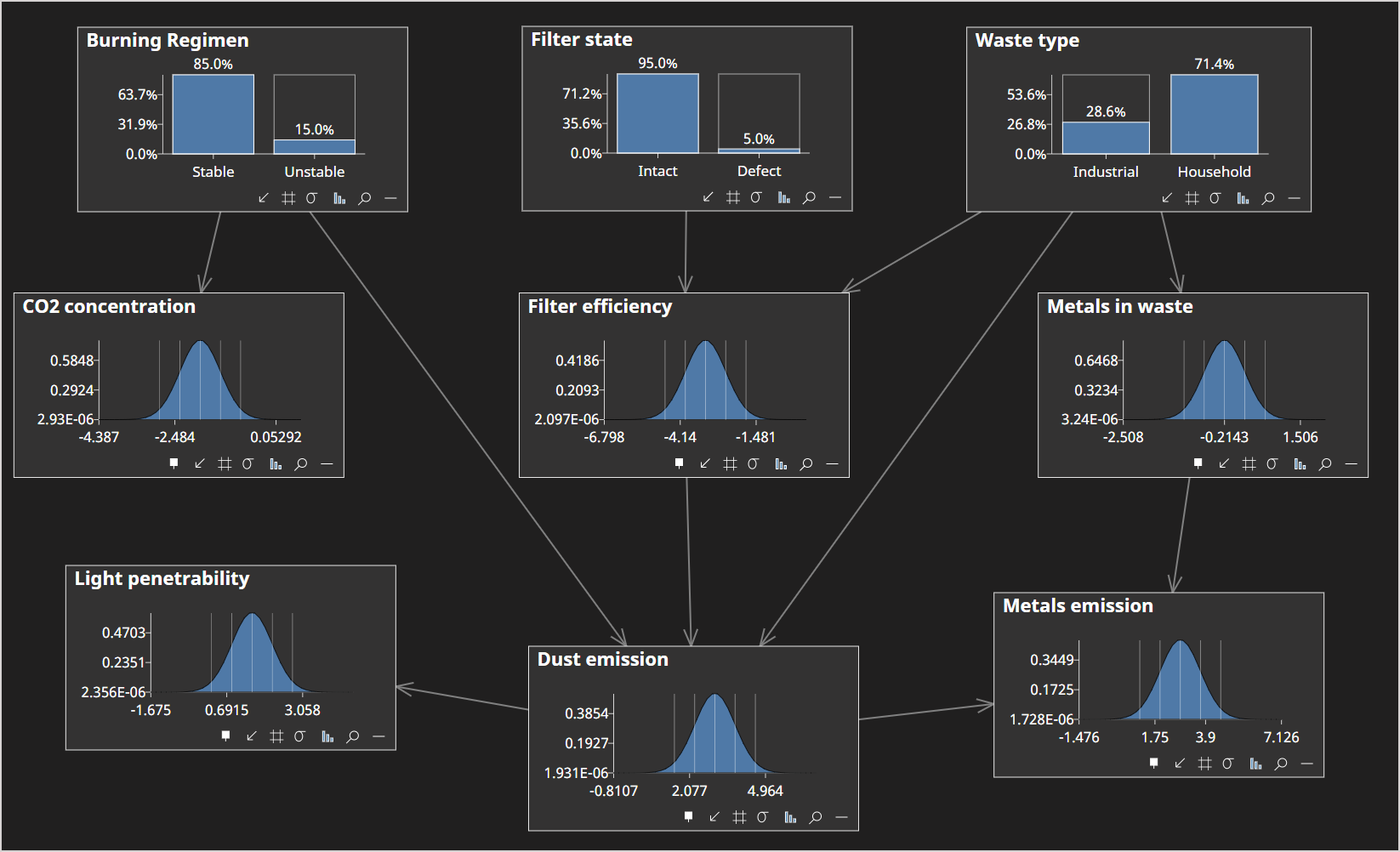
The Waste network with no evidence set should look like this...

• Enter the following evidence, by clicking in the respective node's chart area:

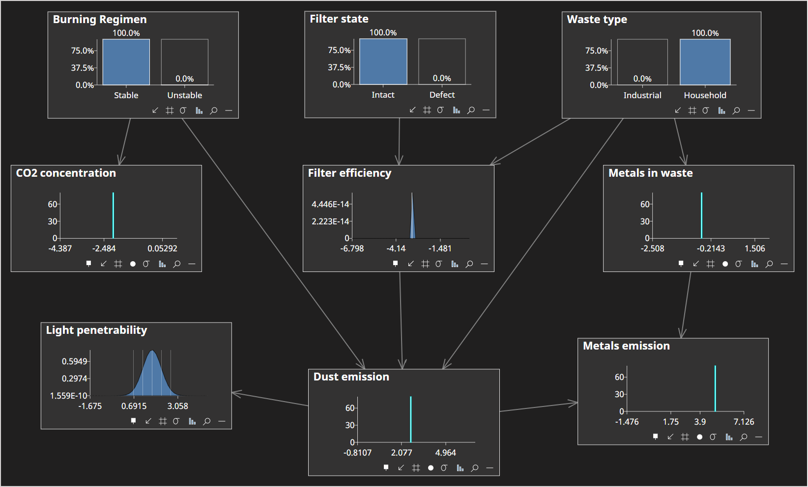
  • Dust emission = 2.66313985
  • CO2 concentration = -2.083988057
  • Metals in waste = -0.582229045
  • Metals emission = 5.015586618

The network should look as follows:

• From the Analyze menu click Likelihood and then Log-Likelihood.

The Log-Likelihood dialog is displayed and should look as follows:

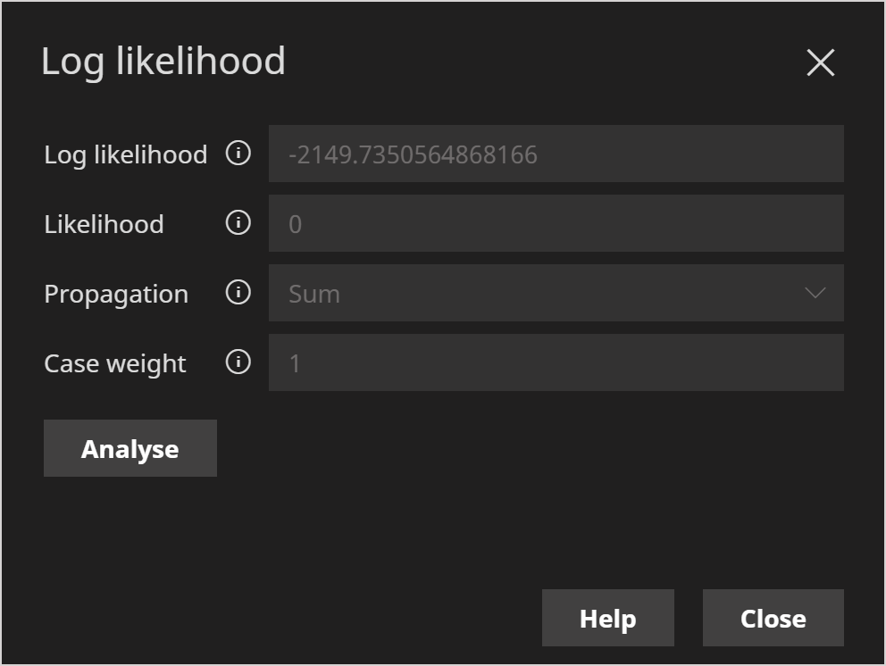
The reported log-likelihood of -2149.73 is quite low, indicating that this evidence is unusual / anomalous.

info

To help understand what values are normal, we can use Data Sampling to generate samples from the network, followed by a Batch query outputting the log-likelihood. We could then plot these values to get a sense of the range of normal values, or see Log-Likelihood for information on how to build an empirical histogram density from which the cdf and inverseCdf can be calculated, which is a more analytical approach.

info

We could also click Analyze to perform a Log-likelihood analysis which helps us understand which variable(s) are contributing most to a low log-likelihood values. This will be covered to a separate tutorial.

Part 2 - Batch log-likelihood query

In part 2 of this tutorial, rather than considering a single query as in part 1, we will cover how to calculate the log-likelihood for an entire dataset.

info

A further related analysis tool is the Retracted analysis tool which helps us understand whether data (and which variables) is anomalous or not. This will be covered to a separate tutorial.

• Download the data for this part of the tutorial from Waste Anomaly Detection data

info

The data included in this file has 400 data points over 4 different variables. The first 300 data points are 'normal' after which the system starts to degrade over the remaining 100.

• Open the file just downloaded in a spreadsheet application.

• Create a line chart for each of the following columns:

  • CO2 Concentration
  • Dust emission
  • Metals emission
  • Metals in waste

The line chart for CO2 Concentration, for example, should look similar to the following:

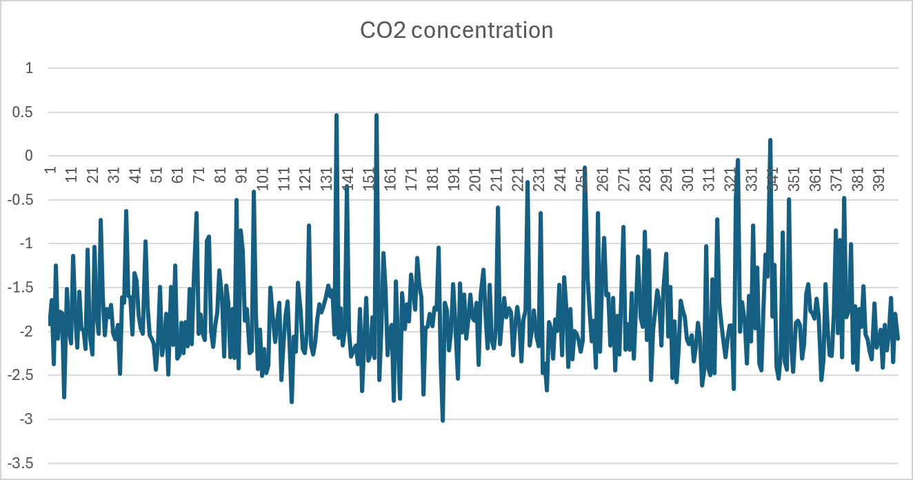
• Verify that for each line chart, while there is variability, there is no obvious indicator that the system is degrading over the last 100 points.

• With the Waste network still open, click the Query menu and then Batch.

The Data Tables dialog will launch as shown below:

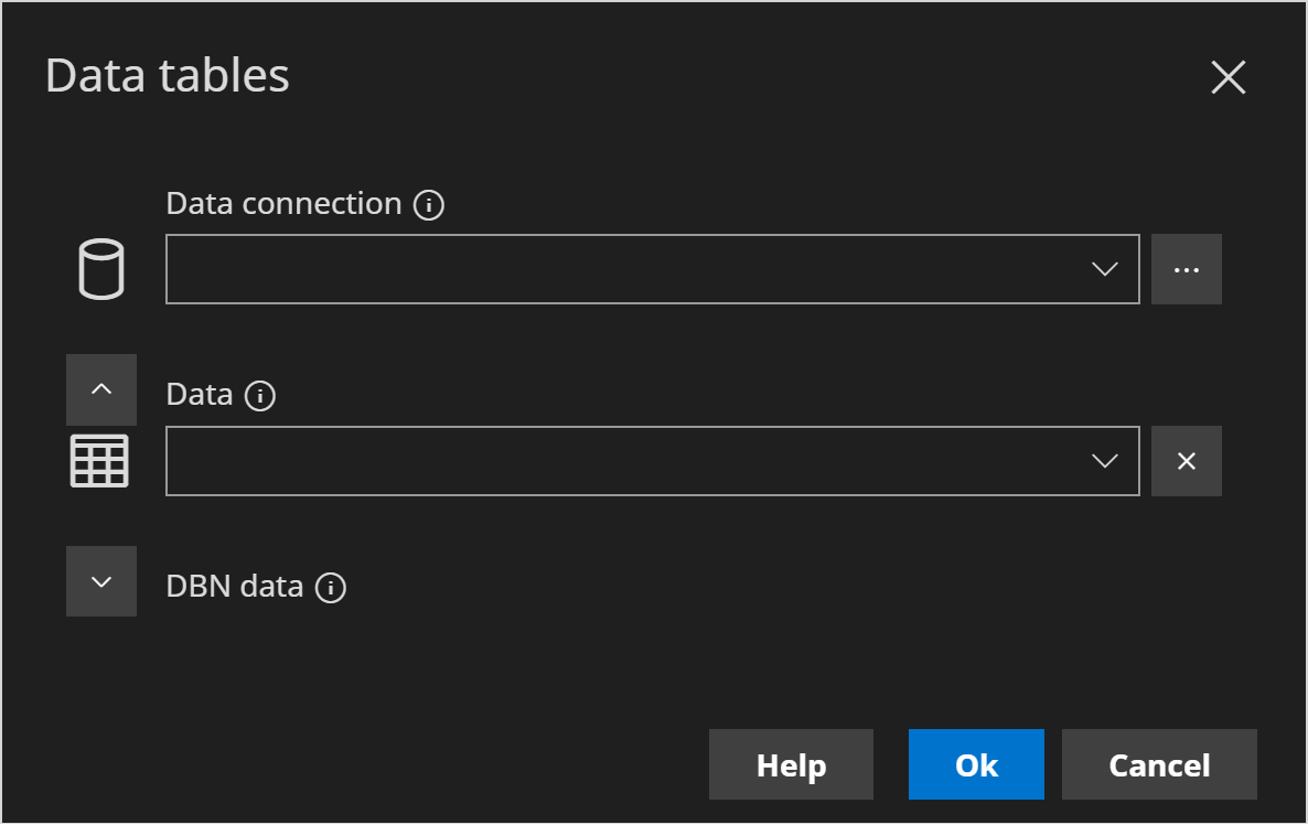
• Click the ellipsis (...) button to the right of the Data Connection drop down.

• Click Add

• With the Load Excel file into memory tab selected, click Open File and select the file you just downloaded.

The New Data Connection dialog should as follows:

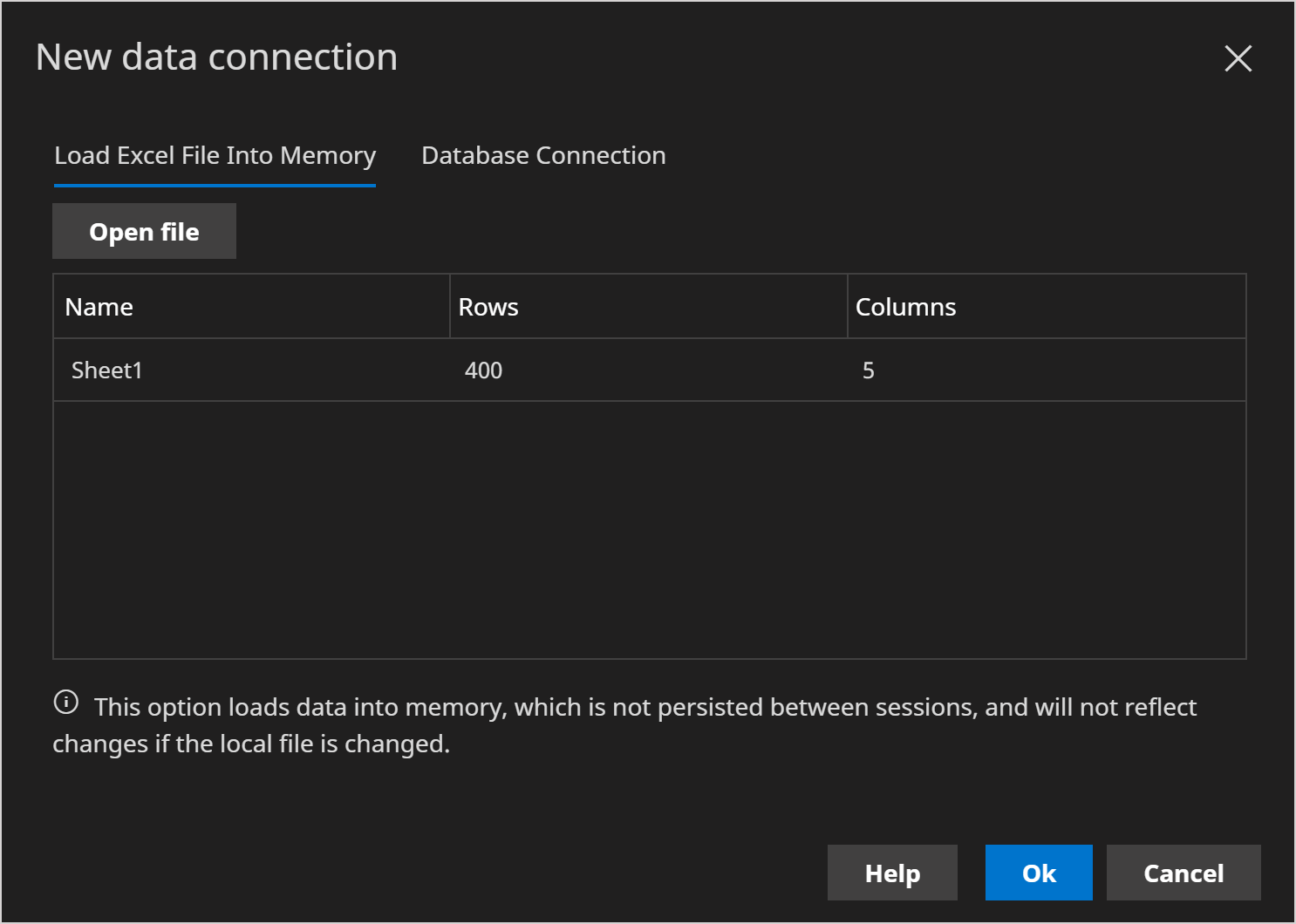
• Click OK to close the dialog.

• Click Close to close the Data Connection Manager.

• In the Data Tables dialog, choose the data connection just created, from the Data Connection drop down.

• Then choose Sheet1 in the Data drop down.

The dialog should look as follows:

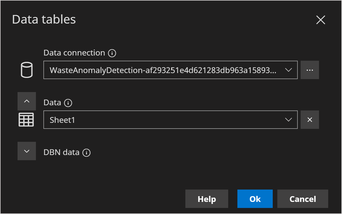
• Click Ok. This will launch the Data Map dialog shown below.

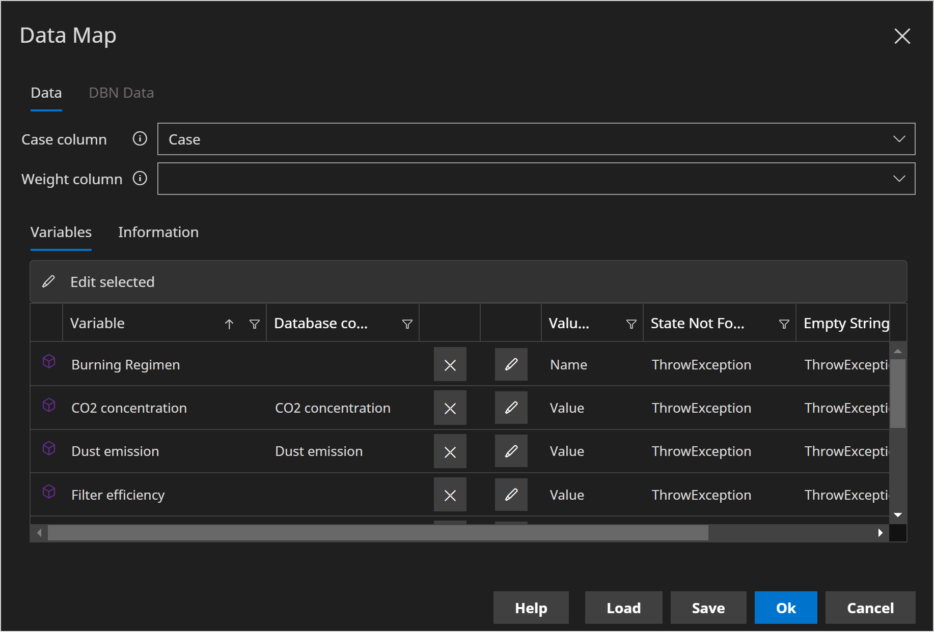
• Check that the following 4 variables have been automatically mapped.

  • CO2 Concentration
  • Dust emission
  • Metals emission
  • Metals in waste

• Click Ok. This will launch the Batch query dialog.

• Check Log Likelihood.

The dialog should look as follows:

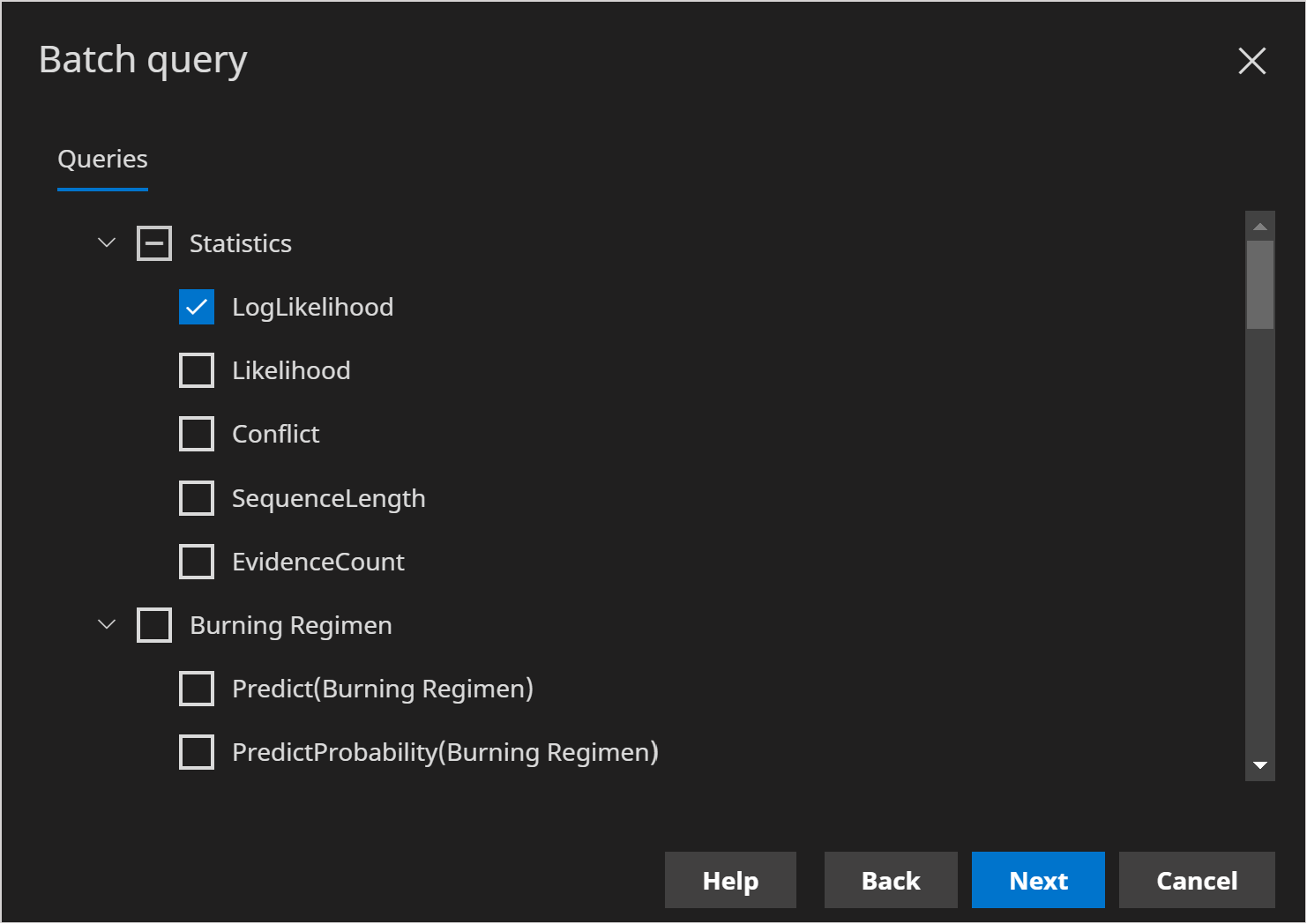
• Click Next. We will leave all the options as defaults.

• Click Next.

• Click Run. The results dialog should look as follows:

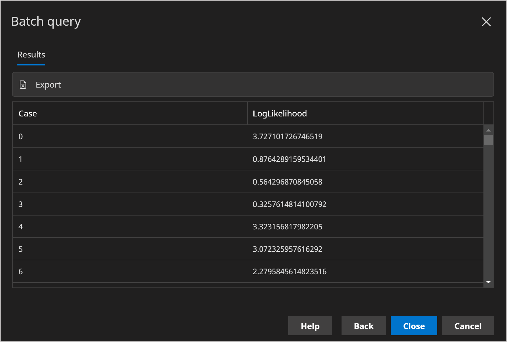
At this point, we have calculated the log-likelihood for all 400 rows in the data source.

• Click Export and save to a file called WasteBatchLogLikelihood.xlxs.

• Open the file just created in a spreadsheet application such as Microsoft Excel.

• Create a scatter chart of the LogLikelihood column.

It should look similar to the following:

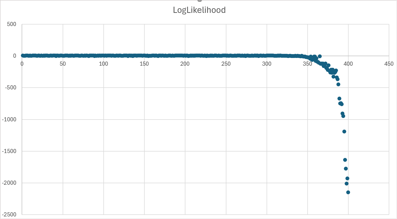
• Verify that the log-likelihood is clearly degrading over the last 100 points, even though each variable when viewed in isolation does not clearly show this.

info

A companion tool to help understand anomalous behavior over a data set is the Retracted Analysis.